

Minimizing remote storage usage and synchronization time using deduplication and multichunking: Syncany as an example
Contents
Download as PDF: This article is a web version of my Master’s thesis. Feel free to download the original PDF version.
3. Deduplication
Since the core algorithms of Syncany strongly rely on deduplication, this chapter introduces the fundamental concepts known in this research area. The first part defines the term and compares the technique to other storage reducing mechanisms. The subsequent sections introduce different deduplication types and elaborate on how success is measured.
3.1. Overview
Data deduplication is a method for maximizing the utility of a given amount of storage. Deduplication exploits the similarities among different files to save disk space. It identifies duplicate sequences of bytes (chunks) and only stores one copy of that sequence. If a chunk appears again in the same file (or in another file of the same file set), deduplication only stores a reference to this chunk instead of its actual contents. Depending on the amount and type of input data, this technique can significantly reduce the total amount of required storage [41,42,45].
For example: A company backs up one 50 GB hard disk per workstation for all of its 30 employees each week. Using traditional backup software, each workstation either performs a full backup or an incremental backup to the company’s shared network storage (or to backup tapes). Assuming a full backup for the first run and 1 GB incremental backups for each workstation per week, the totally used storage after a three months period is 1,830 GB of data.1 Using deduplication before storing the backups to the network location, the company could reduce the required storage significantly. If the same operating system and applications are used on all machines, there is a good chance that large parts of all machines consist of the same files. Assuming that 70% of the data are equal in the first run and 10% of the 1 GB incremental data is identical among all workstations, the totally required storage after three months is about 510 GB.2
While this is just an example, it shows the order of magnitude in which deduplication techniques can reduce the required disk space over time. The apparent advantage of deduplication is the ability to minimize storage costs by storing more data on the target disks than would be possible without it. Consequently, deduplication lowers the overall costs for storage and energy due to its better input/output ratio. Unlike traditional backups, it only transfers new file chunks to the storage location and thereby also reduces the bandwidth consumption significantly. This is particularly important if the user upload bandwidth is limited or the number of backup clients is very high.
Another often mentioned advantage is the improved ability to recover individual files or even the entire state of a machine at a certain point in time. In tape based backups, the restore mechanism is very complex, because the backup tape needs to be physically rewound to get the desired files. Using incremental backups on regular hard disks, the files of a given point in time may be split among different increments and hence needs to be gathered from various archives to be restored. In contrast, the restore mechanism in deduplication systems is rather simple. The index provides a file and chunk list for each backup, so restoring a file set is simply a matter of retrieving all chunks and assembling them in the right order.
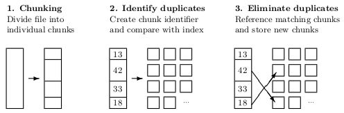 |
| Figure 3.1: Generic deduplication process (according to [35]). |
Figure 3.1 illustrates the generic deduplication process in three simple steps. In step 1, a file is broken into individual chunks. This can be done using fixed-size steps or variable-size chunking methods. In step 2, each of these chunks is then hashed to create a unique chunk identifier using a checksum algorithm such as MD5 or SHA-1. These identifiers are then looked up in the chunk index — a database that stores chunk identifiers and their mapping to the individual files. In step 3, chunks that already exist in the index are referenced to the current file and new chunks are added to the index.
3.2. Distinction and Characteristics
Similar to compression, deduplication encodes data to minimize disk usage. However, while compression is typically local to a file set or tree, deduplication is not bound to the location of a file on a disk or the date and time it is indexed. Compression mechanisms such as Lempel-Ziv (LZ) or Deflate have no persistent dictionary or index outside the created archive file. Once the compression algorithm is terminated, the index is written to the archive file and then purged from the memory. In contrast, deduplication follows a more stateful approach. Every chunk that a deduplication algorithm encounters is looked up in a global chunk index which is kept in the operating system’s memory or in a database. Depending on the use case, this index might even be distributed among different computers.
Unlike compression algorithms, deduplication does not describe exact algorithms to encode data in a certain way. Instead, it rather describes the general mechanisms, processes and design considerations. Deduplication does not have any standardized widely spread algorithms (such as LZ77 or PKZIP in data compression), but rather points out where, when and how it occurs. This particularly includes the following aspects [40,35]:
- Location: Deduplication can be performed at different locations. Depending on the participating machines and steps in the customized deduplication process, it is either performed on the client machine (source-side) or near the final data store (target-side). In the former case, duplicates are removed before the data is transmitted to its storage. Since that conserves network bandwidth, this option is particularly useful for clients with limited upload bandwidth. However, since deduplication needs to analyze each file very closely, it can significantly increase the load on the client CPU. In the latter case, the chunking and indexing is done on the server and hence does not consume processing time on the client, but on the server machine. Since this method potentially transfers duplicate data, it is only acceptable if the client’s upload bandwidth is sufficient.
- Time: Depending on the use case, deduplication is either performed as the data is transferred from the source to the target (in-band or in-line) or asynchronously in well-defined intervals (out-of-band or post-process). In the former case, data written to the target storage does not contain any duplicate chunks. Duplicates are identified and eliminated on the client or server as part of the data stream from source to target. In out-of-band deduplication systems on the other hand, the original data is written to the server storage and only later cleaned from duplicates. The in-band approach requires no post-processing and minimizes the required storage immediately. However, depending on the amount of data, this approach can cause a bottleneck in terms of throughput on the server side. Even though the out-of-band approach solves the bottleneck problem, it needs to buffer the undeduplicated data for the time between the deduplication runs. That is the server potentially needs multiple times the amount of disk space just so it can retain duplicate data.
- Chunking method: Deduplication breaks files into small chunks in order to detect duplicates. The method used for chunking largely influences the deduplication success and can also affect the user experience. Literature differentiates four distinct cases [35,42,43,61]: Whole file chunking treats entire files as chunks (independent of their size), fixed-size chunking defines chunk boundaries by fixed offsets, variable-size chunking uses fingerprinting algorithms to determine the chunk boundaries and format-aware chunking (or file type aware chunking) handles files differently according to their file type. Details on these methods are discussed in section 3.4.
- Identifying duplicate chunks: To save storage space, deduplication references redundant data instead of copying its contents. This concept relies on the assumption that each individual chunk has its own identity, i.e. an identifier by which it can be unambiguously referenced. For each chunk of a file, this identifier is calculated and compared to the global chunk index. If a chunk with a matching identifier is found in the database, the two chunks are assumed to be identical and the existing chunk is referenced. If not, the new chunk is added to the index. That is if two chunk identifiers are identical, the contents of the two chunks are also assumed to be identical. Depending on the number space of the chunk identifiers, this assumption can more or less likely lead to false matches and hence to data corruption.
- False matches: Since the identifier is a representation of the chunk contents, deduplication systems typically use cryptographic hash functions such as MD5 or SHA-1 to calculate the chunk identity [8]. Even though hash functions do not entirely eliminate the threat of false matches, they reduce the probability of collisions by equally distributing the identifiers among the according number space. The greater the number space, i.e. the more bits in the chunk identifier, the smaller is the chance of collisions. If, for instance, the 128-bit hash function MD5 is used on a dataset of 1 TB with a chunk size of 8 KB, the chance of one chunk ID collision is about 2.3 × 10⁻²³. For the 160-bit SHA-1 function, this probability is only 5.3 × 10⁻³³. The collision chance is 50% or greater if 32 TB of data are analyzed (for MD5) or 2.1 × 106 TB (for SHA-1) respectively.3 Depending on the amount of data to be stored, the hash collision problem might be an issue or not. While hash functions that create long hashes (e.g. SHA-512 or Whirlpool) are typically preferred to reduce the possibility of false matches, shorter hashes are more desirable when the size of the index or the processing time is an issue. The selection of the hash function is hence strongly application dependent.
3.3. Applications
Due to its storage-reducing nature, deduplication is almost exclusively used for backup systems and disaster recovery. Commercial products are mainly targeted at medium to large companies with a well-established IT infrastructure. Deduplication-based archive systems are available as both software and hardware. Software-based deduplication systems are typically cheaper to deploy than the hardware-based variant, because no changes to the physical IT landscape are necessary. However, the software variant often requires installing agents on all workstations and is hence more difficult to maintain. Hardware based systems on the other hand are known to be more efficient and to scale better. Once integrated in the IT infrastructure, they are often mounted as file systems to make the deduplication process transparent to applications. On the contrary, they are only suitable for target based deduplication and can hence not save network bandwidth [64,65].
Pure software implementations are typically either directly embedded into the backup software or are available as standalone products and can be installed between the backup application and the storage device. Examples for the first case include the IBM Tivoli Storage Manager (TSM) [35] and Acronis Backup & Recovery. Both pieces of software include their own deduplication mechanisms. Since version 6, TSM provides both source and target deduplication and all operations are performed out-of-band. Acronis provides similar features. Examples for standalone deduplication software include EMC Corp.’s Data Domain Boost or Symantec NetBackup PureDisk (was at: www.symantec.com/business/netbackup-puredisk, now defunct, July 2019).
Hardware-based systems are available in different configurations. They mainly differ in the throughput they can handle as well as in whether they process data in-band or out-of-band. Popular solutions are the Data Domain DDx series [7] and the ExaGrid EX series [5]. Data Domain offers appliances from 430 GB/hour up to 14.7 TB/hour. It processes data in-band and maintains the chunk index in nonvolatile RAM. ExaGrid’s solution uses out-of-band data deduplication, i.e. it post-processes data after it has been written to the Landing Zone and only later writes it to the final storage. ExaGrid’s systems offer a throughput of up to 2.4 TB/hour.
3.4. Chunking Methods
As briefly mentioned in section 3.2, deduplication greatly differs in how redundant data is identified. Depending on the requirements of the application and the characteristics of the data, deduplication systems use different methods to break files into individual chunks. These methods mainly differ in the granularity of the resulting chunks as well as their processing time and I/O usage.
Chunking methods that create coarse-grained chunks are generally less resource intensive than those that create fine-grained chunks. Because the resulting amount of chunks is smaller, the chunk index stays relatively small, fewer checksums have to be generated and fewer ID lookups on the index have to be performed. Consequently, only very little CPU is used and the I/O operations are kept to a minimum. However, bigger chunk sizes have a negative impact on their redundancy detection and often result in less space savings on the target storage.
Conversely, fine-grained chunking methods typically generate a huge amount of chunks and have to maintain a large chunk index. Due to the excessive amount of ID lookups, the CPU and I/O load is relatively high. However, space savings with these methods are much higher.
The following sections introduce the four most commonly used types of deduplication and discuss their advantages and disadvantages.
3.4.1. Single Instance Storage
Single instance storage (SIS) or whole file chunking does not actually break files into smaller chunks, but rather uses entire files as chunks. In contrast to other forms of deduplication, this method only eliminates duplicate files and does not detect if files are altered in just a few bytes. If a system uses SIS to detect redundant files, only one instance of a file is stored. Whether a file already exists in the shared storage is typically detected by the file’s checksum (usually based on a cryptographic hash function such as MD5 or SHA-1).
The main advantages of this approach are the indexing performance, the low CPU usage as well as the minimal metadata overhead: Instead of potentially having to create a large amount of chunks and checksums for each file, this approach only saves one checksum per file. Not only does this keep the chunk index small, it also avoids having to perform CPU and I/O intensive lookups for each chunk. On the other hand, the coarse-grained indexing approach of SIS stores much more redundant data than the sub-file chunking methods. Especially for large files that change regularly, this approach is not suitable. Instead of only storing the altered parts of the file, SIS archives the whole file.
The usefulness of SIS strongly depends on the application. While it might not be useful when backing up large e-mail archives or database files, SIS is often used within mail servers. Microsoft Exchange, for instance, used to store only one instance of an e-mail (including attachments) if it was within the managed domain. Instead of delivering the e-mail multiple times, they were only logically referenced by the server.4
3.4.2. Fixed-Size Chunking
Instead of using entire files as smallest unit, the fixed-size chunking approach breaks files into equally sized chunks. The chunk boundaries, i.e. the position at which the file is broken up, occur at fixed offsets — namely at multiples of the predefined chunk size. If a chunk size of 8 KB is defined, a file is chunked at the offsets 8 KB, 16 KB, 24 KB, etc. As with SIS, each of the resulting chunks are identified by a content-based checksum and only stored if the checksum does not exist in the index.
This method overcomes the apparent issues of the SIS approach: If a large file is changed in only a few bytes, only the affected chunks must be re-indexed and transferred to the backup location. Consider a virtual machine image of 5 GB which is changed by a user in only 100 KB. Since the old and the new file have different checksums, SIS stores the entire second version of the file — resulting in a total size of 10 GB. Using fixed-size chunking, only ⌈100 KB / 8 KB⌉ × 8 KB = 104 KB of additional data have to be stored.
However, while the user data totals up to 5 GB and 104 KB, the CPU usage and the amount of metadata is much higher. Using the SIS method, the new file is analyzed by the indexer and the resulting file checksum is looked up in the chunk index, i.e. only a single query is necessary. In contrast, the fixed-size chunking method must generate ⌊5 GB / 8 KB⌋ = 625,000 checksums and perform the same number of lookups on the index. In addition to the higher load, the index grows much faster: Assuming 40 bytes of metadata per chunk, the chunk index for the 5 GB file has a size of (625,000 × 40 bytes) / 109 = 25 MB.
While the fixed-size chunking method performs quite well if some bytes in a file are changed, it fails to detect redundant data if some bytes are inserted or deleted from the file or if it is embedded into another file. Because chunk boundaries are determined by offset rather than by content, inserting or deleting bytes changes all subsequent chunk identifiers. Consider the example from above: If only one byte is inserted at offset 0, all subsequent bytes are moved by one byte — thereby changing the contents of all chunks in the 5 GB file.
3.4.3. Variable-Size Chunking
To overcome this issue, variable-size chunking does not break files at fixed offsets, but based on the content of the file. Instead of setting boundaries at multiples of the predefined chunk size, the content defined chunking (CDC) approach [37] defines breakpoints where a certain condition becomes true. This is usually done with a fixed-size overlapping sliding window (typically 12-48 bytes long). At every offset of the file, the contents of the sliding window are analyzed and a fingerprint, f, is calculated. If the fingerprint satisfies the break-condition, a new breakpoint has been found and a new chunk can be created. Typically, the break-condition is defined such that the fingerprint can be evenly divided by a divisor D, i.e. f mod D = r with 0 ≤ r < D, where typically r = 0 [14,34].
Due to the fact that the fingerprint must be calculated for every offset of the file, the fingerprinting algorithm must be very efficient. Even though any hash function could be used, most of them are not fast enough for this use case. Variable-size chunking algorithms typically use rolling hash functions based on the Rabin fingerprinting scheme [99] or the Adler-32 checksum [98]. Compared to most checksum algorithms, rolling hash functions can be calculated very quickly. Instead of re-calculating a checksum for all bytes of the sliding window at each offset, they use the previous checksum as input value and transform it using the new byte at the current position.
The greatest advantage of the variable-size chunking approach is that if bytes are inserted or deleted, the chunk boundaries of all chunks move accordingly. As a result, fewer chunks have to be changed than in the fixed-size approach. Consider the example from above: Assuming that the 100 KB of new data were not updated in the original file, but inserted at the beginning (offset 0). Using the fixed-size approach, subsequent chunks change their identity, because their content is shifted by 100 KB and their boundaries are based on fixed offsets. The resulting total amount would be about 10 GB (chunk data of the two versions) and 50 MB (metadata). The variable-size approach breaks the 100 KB of new data into new chunks and detects subsequent chunks as duplicates — resulting in only about 100 KB of additional data.
While the fixed-size approach only allows tweaking the chunk size, the variable-size chunking method can be varied in multiple parameters. The parameter with the biggest impact on performance is the fingerprinting algorithm, i.e. algorithm by which the chunk boundaries are detected. The following list gives an overview over the existing well-known mechanisms and their characteristics:
- Rabin: Rabin fingerprints [99] are calculated using random polynomials over a finite field. They are the polynomial representation of the data modulo a predetermined irreducible polynomial [36]. As input parameters for the checksum calculation, a user-selected irreducible polynomial in the form of an integer is used. Because the resulting fingerprints are based on the previous ones, they can be calculated very efficiently. Due to the detailed mathematical analysis of its collision probability, the Rabin scheme (and variations of it) are often used by file systems, synchronization algorithms and search algorithms [36,48,43,34].
- Rolling Adler-32: The rsync synchronization tool uses a rolling hash function which is based on the Adler-32 checksum algorithm [44]. Adler-32 concatenates two separately calculated 16-bit checksums, both of which are solely based on the very efficient add-operation. To the best of the author’s knowledge, the Adler-32 algorithm has not been used in commercial or non-commercial deduplication systems before.
- PLAIN: Spiridonov et. al [38] introduce the Pretty Light and Intuitive (PLAIN) fingerprinting algorithm as part of the Low Bandwidth File System. Similar to Adler-32, PLAIN is based on additions and is hence faster to compute than Rabin. They argue that the randomization (as done in Rabin) is redundant, because the data on which the algorithm is applied can be assumed to be fairly random. By eliminating the randomization, the algorithm speed is superior to the Rabin hash function.
All of the above mentioned fingerprinting algorithms can be part of any given variable-size chunking method. The simplest method is the basic sliding window (BSW) approach (as used in the LBFS) [36]: BSW entirely relies on the fingerprinting algorithm to determine chunk boundaries and breaks the file only if the break condition matches. While this produces acceptable results in most cases, it does not guarantee a minimum or maximum chunk size. Instead, chunk boundaries are defined based on the probability of certain fingerprints to occur. Depending on the divisor D and the size of the sliding window, this probability is either lower or higher: The smaller the value of D, the higher the probability that the checksum is evenly divisible. Similarly, the bigger the size of the sliding window, the lower the probability.
Even if the chunk size is expected to be in a certain range for random data, non-random data (such as long sequences of zeros) might cause the break condition to never become true. Consequently, chunks can grow infinitely if no maximum chunk size is defined. Similarly, if the break condition matches too early, very small chunks might be created.
In contrast to BSW, there are other variable-size chunking methods that handle these special cases:
- The Two Threshold Two Divisor (TTTD) chunking method [39] makes sure that it does not produce chunks smaller than a certain threshold. To do so, it ignores chunk boundaries until a minimum size is reached. Even though this negatively affects the duplicate detection (because bigger chunks are created), chunk boundaries are still natural — because they are based on the underlying data. To handle chunks that exceed a certain maximum size, TTTD applies two techniques. It defines the two divisors D (regular divisor) and D’ (backup divisor) with D > D’. Because D’ is smaller than D, it is more likely to find a breakpoint. If D does not find a chunk boundary before the maximum chunk size is reached, the backup breakpoint found by D’ is used. If D’ also does not find any breakpoints, TTTD simply cuts the chunk at the maximum chunk size. TTTD hence guarantees to emit chunks with a minimum and maximum size.
- The algorithm proposed by Kruus et. al [37] instead uses chunks of two different size targets. Their algorithm emits small chunks in limited regions of transition from duplicate to non-duplicate data and bigger chunks elsewhere. This strategy assumes that (a) long sequences of so-far unknown data have a high probability of re-appearing in later runs and that (b) breaking big chunks into smaller chunks around change regions will pay off in later runs. While this strategy might cause data to be stored in both big and small chunks, the authors show that it increases the average chunk size (and hence reduces metadata) while keeping a similar deduplication elimination ratio.
Assuming an average chunk size equal to the fixed-size chunking approach, variable-size methods generate roughly the same amount of metadata and are only slightly more CPU intensive.
3.4.4. File Type Aware Chunking
All of the above chunking methods do not need any knowledge about the file format of the underlying data. They perform the same operations independent of what the data looks like. While this is sufficient in most cases, the best redundancy detection can be achieved if the data stream is understood by the chunking method. In contrast to other methods, file type aware chunking knows how the underlying data is structured and can hence set the chunk boundaries according to the file type of the data.
The advantages are straightforward: If the chunking algorithm is aware of the data format, breakpoints are more natural to the format and thereby potentially facilitate better space savings. Consider multimedia files such as JPEG images or MP3 audio files: Using a file type unaware chunking algorithm, some of the resulting chunks will most probably contain both metadata and payload. If the metadata changes (in this case Exif data and ID3 tags), the new chunks will again contain metadata and the identical payload, i.e. redundant data is stored in the new chunks. Using a file type aware chunking method, chunk boundaries are set to match logical boundaries in the file format. In this case, between the metadata and the payload, so that if only the metadata changes, the payload will never be part of new chunks.
If the file format is known, it is also possible to adjust the chunk size depending on the section of a file. For some file formats (or file sections), it is possible to make assumptions on how often they are going to be changed in the future and vary the chunk size accordingly. A rather simple strategy for multimedia files, for instance, could be to emit very small chunks (e.g. ≤ 1 KB) for the metadata section of the file and rather big chunks for the actual payload (e.g. ≥ 512 KB) — assuming that the payload is not likely to change as often as the metadata. In this example, the result would be significantly fewer chunks (and thereby also fewer chunk metadata) than if the whole file would be chunked with a target chunk size of 8 KB.
Other examples for potential chunk boundaries include slides in a PowerPoint presentation or pages in a word processing document. As Meister and Brinkmann [68] have shown, understanding the structure of composite formats such as TAR or ZIP archives can lead to significant space savings. Both ZIP and TAR precede all file entries with a local header before the actual data. Since many archive creators change these headers even if the payload has not changed, the resulting archive file (after a minor change in a single file) can differ significantly. Understanding the archive structure and setting the chunk boundaries to match metadata and payload boundaries invalidates smaller chunks and avoids having to store duplicate data.
However, even if the advantages are numerous, the approach also implies certain disadvantages. The most obvious issue of the file type aware chunking method is the fact that in order to allow the algorithm to differentiate among file formats, it must be able to understand the structure of each individual type. Ideally, it should support all of the file formats it encounters. Due to the enormous amount of possible formats, however, this is not a realistic scenario. Many file formats are proprietary or not well documented which sometimes makes it necessary to reverse-engineer their structure — which obviously is very costly. Instead of trying to understand them all, supporting only those that promise the most space savings can be a way to achieve a good trade-off.
Another issue arises from the fact that when type-dependent chunks are created, the chunking method might not detect the same data if it appears in another file format. If, for instance, an MP3 audio file is broken into chunks using an MP3-specific chunking algorithm, the payload data might not be detected as duplicate if it appears in a TAR archive or other composite formats. In some cases, the type-specific algorithms might hence negatively affect the efficiency of the chunking algorithm.
While file type aware chunking bears the greatest potential with regard to space savings, it is certainly the most resource intensive chunking method. Due to the detailed analysis of the individual files, it typically requires more processing time and I/O usage than the other methods [35, 61].
3.5. Quality Measures
In order to compare the efficiency of the above-mentioned chunking methods, there are a few quality metrics that are often used in literature as well as in commercial products. The following sections introduce the most important tools to evaluate these methods.
3.5.1. Deduplication Ratio
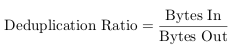
By far the most prominent measure is the deduplication ratio (also: data elimination ratio (DER) [38] or fold factor [40]), a value that measures the space savings achieved through the deduplication mechanisms. It is calculated by dividing the number of input bytes (before deduplication) by the number of output bytes (after deduplication) [42]:
 |
(3.1) |
Depending on how many redundant bytes are eliminated in the deduplication process, the ratio is either higher or lower. Higher values either indicate more effective redundancy elimination or a greater amount of redundant data in the input bytes. Lower values conversely point towards less efficiency in the duplicate detection or fewer redundant bytes in the input. Depending on whether or not the deduplication metadata is included when counting the number of output bytes, the ratio might even become lower than one. In this case, i.e. if there are more output bytes than input bytes, the deduplication process is not only inefficient, but generates additional data. Even though this is a rare case, it can happen if the input data has no or very little redundant data.
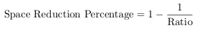
The ratio is typically written as ratio:1, indicating that ratio input bytes have been transformed to one output byte by the deduplication process. Another way to express the space savings is to transform the ratio into the space reduction percentage, i.e. the percentage of how much disk space has been saved through the deduplication process. It is calculated as 100% less the inverse of the space reduction ratio [42]:
 |
(3.2) |
Continuing the example of the company with 30 workstations from section 3.1, the space reduction ratio for the first full backup run is (1,500 GB / 450 GB) ≈ 3.3:1 and the space reduction percentage is 70%. After the total three months period of weekly incremental backups, this ratio rises up to about 3.6:1 and the space reduction percentage up to 72%. If the company were to do full backups instead of incremental backups every week, the ratio would be significantly higher.
The space reduction ratio and percentage do not only depend on the chunking method and fingerprinting algorithms, but also on factors that can only be marginally influenced (if at all). Depending on these factors, the efficiency of deduplication greatly varies and might (in rare cases) even have negative effects on the storage usage. Among others, this includes the following factors (largely based on [42]):
- Data type: The type of the data stored by workstation users has by far the greatest impact on the deduplication ratio. Depending on how original the users’ files are, i.e. whether or not the corresponding chunks are present in the chunk index, deduplication is more or less effective. If, for instance, a group of users only changes few parts of the same set of files every day, the deduplication effect is certainly much higher than if they create new files regularly.
For compressed or encrypted data, deduplication typically has no or very little effect, because the compressed/encrypted data often changes significantly even if only a few bytes in the source data are changed. - Data change frequency: The rate by which data is changed on the users’ workstations does not have a direct influence on the deduplication ratio, but rather on the probability of redundant data to occur. The more often files are changed or new files are added, the higher is the probability that unique data has been generated. That means that in general, the deduplication ratio decreases when the data change frequency increases.
- Data retention period: The time for which the deduplicated data (and the corresponding chunk index) is stored can affect the deduplication ratio. The longer backups are stored, the greater the amount of unique chunks tends to become. It is hence more likely to find duplicates if the retention period is longer.
3.5.2. Metadata Overhead
Even though the deduplication ratio is often the only measure by which commercial deduplication providers advertise their solutions, other factors are often as important.
The metadata overhead describes the amount of extra data that needs to be maintained by the deduplication system to allow the reconstruction of files and to enable duplicate detection. In particular, this includes a list of the deduplicated files as well as a list of what chunks these files are compiled of. The actual amount of metadata strongly depends on the size of the chunk fingerprint as well as the target chunk size. The more bits a fingerprint consists of and the smaller the average chunk size, the more metadata has to be maintained (and transferred) by the system.
Apart from the total overhead for a particular file set, the metadata overhead is often expressed as per-chunk overhead or overhead per-megabyte [37,42]. The per-chunk overhead is the extra data that needs to be stored for each individual chunk. Its values are typically in the range of twenty to a few hundred bytes [37] — depending on the fingerprint size and what other data is stored in the system. The overhead per megabyte is the average cost for each megabyte of the deduplicated data. Its value is defined by Kruus et al. as metadata size divided by the average chunk size.
Typically, the total size of the metadata is not relevant compared to the amount of space savings it enables. However, in cases in which it exceeds the system’s memory, it can have enormous impact on the performance of the deduplication software. Once the chunk index has become too big to be stored in the memory, the chunking algorithm has to perform costly disk operations to lookup the existence of a chunk. Particularly in large enterprise-wide backup systems (or in other scenarios with huge amounts of data), this can become a serious problem. Assuming a per-chunk overhead of 40 bytes and an average chunk size of 8 KB, 1 GB of unique data creates 5 MB of metadata. For a total amount of a few hundred gigabytes, keeping the chunk index in the memory is not problematic. For a total of 10 TB of unique data, however, the size of the chunk index is 50 GB — too big even for large servers.
The solutions suggested by the research community typically divide the chunk index into two parts: One part is kept in the memory and the other one on the disk. Zhu et al. [69] introduce a summary vector, a method to improve sequential read operations on the index. Bhagwat et al. [14] keep representative chunks in the memory index and reduce the disk access to one read operation per file (instead of one per chunk). Due to the fact that these solutions are often limited to certain use cases, many deduplication systems have a memory-only chunk index and simply cannot handle more metadata than the memory can hold.
To evaluate the performance of a deduplication system, the importance of the metadata overhead strongly depends on the use case. If the expected size of the chunk index easily fits into the machine’s memory, the metadata overhead has no impact on the indexing performance. However, for source-side deduplication, it still affects the total transfer volume and the required disk space. If the expected size of the chunk index is larger than the memory, the indexing speed (and hence the throughput) slows down by the order of magnitudes [40].
3.5.3. Reconstruction Bandwidth
Reconstruction is the process of reassembling files from the deduplication system. It typically involves looking up all chunks of the target file in the chunk index, retrieving these chunks and putting them together in the right order.
Depending on the type of the system, quickly reconstructing files has a more or less high priority. For most backup systems, only the backup throughput is of high relevance and not so much the speed of reconstruction. Because backups potentially run every night, they must be able to handle large amounts of data and guarantee a certain minimum throughput. Restoring files from a backup, on the other hand, happens irregularly and only for comparatively small datasets.
In most cases, the reconstruction bandwidth is not a decision criterion. However, in systems in which files need to be reassembled as often as they are broken up into chunks, the reconstruction speed certainly matters.
The chunks in a deduplication system are typically stored on the local disk or on a network file system. The reconstruction process involves retrieving all of these chunks individually and thereby causes significant random disk access. Consequently, the average reconstruction bandwidth strongly depends on how many disk reads must be performed. Since the amount of read operations depends on how many chunks a file consists of, the reconstruction bandwidth is a direct function of the average chunk size [40]: If the chunks are small, the system has to perform more disk reads to retrieve all required data and achieves a lower average reconstruction bandwidth. Conversely, bigger chunks lead to a higher reconstruction bandwidth.
While a high amount of disk read operations is not problematic on local disks, it certainly is an issue for distributed file systems or other remote storage services. Considering NFS, for instance, open and read operations are translated into multiple requests that need to be sent over a network. Depending on whether the storage server is part of the local area network or not, a high amount of requests can have significant impact on the reconstruction bandwidth.
Regarding the reconstruction bandwidth, it is beneficial to have large chunks in order to minimize disk and network latency. With regard to achieving a higher deduplication ratio, however, smaller chunks are desirable.
3.5.4. Resource Usage
Deduplication is a resource intensive process. It encompasses CPU intensive calculations, frequent I/O operations as well as often excessive network bandwidth usage. That is each of the steps in the deduplication process has an impact on the resource usage and might negatively affect other applications. Among others, these steps include the following (already discussed) operations:
- Reading and writing files from/to the local disk (I/O)
- Identifying break points and generating new chunks (I/O, CPU)
- Looking up identifiers in the chunk index (I/O, CPU, RAM)
- Creating checksums for files and chunks (CPU)
Resource usage is measured individually for CPU, RAM, disk and network. Typical measures include (but are not limited) to the following:
- CPU utilization measures the usage of the processor. Its values are typically represented as a percentage relative to the available processing power. Values greater than 100% indicate a certain amount of runnable processes that have to wait for the CPU [70].
- The number of CPU cycles represents the absolute number of instruction cycles required by an operation. It is more difficult to measure, but often more comparable amongst different systems.
- Disk utilization measures the device’s read/write saturation relative to the CPU utilization. It is expressed as the percentage of the CPU time during which I/O requests were issued [71].
- The time needed by an operation to terminate (in milliseconds or nanoseconds) can be used to measure its complexity. It is an easy measure, but strongly depends on the system.
- Network bandwidth measures the upload and download bandwidth in MB/s or KB/s. It expresses the speed of the upload and download and often also includes potential latencies of the connection.
- RAM utilization measures the memory used by the application relative to the totally available system memory in percent and/or absolute in MB.
The extent to which each of the system’s available resources is used by the deduplication system depends on several factors. Most importantly, it depends on the location and time of the deduplication process (as discussed in section 3.2): Source-side systems, for instance, perform the deduplication on the client machine and hence need the client’s resources. They do not consume as much network bandwidth as target-side systems. Similarly, if deduplication is performed out-of-band, the resources are not used all the time, but only in certain time slots.
Besides the spatial dimension and the time of execution, resource usage can be influenced by the parameters discussed in the sections above. Among others, it strongly depends on the chunking method, the fingerprinting algorithm and the chunk size. According to literature, particularly the chunk size has a great impact [40], since it has direct implications on the amount of chunk index entries and hash lookups, as well as on the amount of file open operations.
While resource usage is not much of an issue if deduplication is performed by a dedicated machine, it is all the more important if it must be performed in-band on the client’s machine. If this is the case, deduplication cannot disrupt other services or applications and must stay invisible to the user. Since limiting the resource usage often also means lowering the deduplication ratio or the execution time, these elements must be traded off against each other, depending on the particular use case.
- 1 50 GB × 30 workstations in the initial run, plus 11 weeks × 30 workstations × 1 GB in all of the incremental runs.
- 2 50 GB of equal data, plus 30 workstations × 30% × 50 GB in the initial run, plus 11 weeks × 90% × 1 GB in all of the following runs.
- 3 All values are calculated under the assumption that the hash value is distributed equally in the number space. The probability of one collision is calculated using the birthday problem approximation function p(chunk_count, number_space) = 1 – exp(-chunk_count2/(2 × number_space)), with chunk_count being the maximum amount of possible unique chunks in the data set and number_space being the possible hash combinations. The collision chance is calculated in an analog way.
- 4 Due to performance issues, this feature was removed in Microsoft Exchange 2010.
Hi,
I would love to see a ebook version of your thesis (epub or mobi). Would that be possible ?
thanks
@JP: Is there a simple way to compile it from LaTeX format? If it is, I can definitely make one for you. Just let me know :-)
Hi Philipp:
Good Morning. Possible to receive pdf version of your thesis.
cheers
Madhavan